


Scientific research results in pandemic conditions (COVID-19)
174
Mengliyev Sh.A., Doctor of Philosophy in Technical Sciences
Termez State University (Ph.D)
Xamrayev A.B., student of Termez State University
NEWTON'S METHOD OF SOLVING A SYSTEM OF NONLINEAR EQUATIONS
Sh. Mengliyev, A. Xamrayev
Abstract. The concept of a system of nonlinear equations, the stages of
solving the problem, the geometric interpretation of the solution of the
equation and the concept of iterative processes are given and their
application is shown in the examples. The problem of numerical solution of
a number of practical problems consisting of a system of nonlinear
equations is considered. There are a number of approximate computational
methods for solving systems of nonlinear equations, including Newton's
method. Using these methods, a number of specific practical problems were
solved, a computational algorithm and a block diagram were developed. An
approximate method of finding the true roots of a system of nonlinear
equations is given, based on examples, graphs are used in the form of results,
and appropriate conclusions are drawn.
Keywords: System of nonlinear equations, Maple, Newton's method,
algorithm, graph, block diagram, approximate method, geometric
interpretation, iterative process, numerical solution.
Many practical problems lead to the solution of a system of nonlinear
equations. In general, a system of n unknown nonlinear algebraic or
transcendental equations is written as follows:
{
𝑓(x
1
, x
2
, … , x
n
) = 0
𝑓
3
(x
1
, x
2
, … , x
n
) = 0
… … … … … … … … … .
𝑓
n
(x
1
, x
2
, … , x
n
) = 0
(1)
This (1) system can be written in vector form as follows:
𝑓 ( x ) = 0. (2)
here x = (x
1
, x
2
, … , x
n
)
𝑇
– vector column of arguments;
(𝑓
1
, 𝑓
2
, … , 𝑓
n
)
𝑇
– vector column of functions; ( … )
𝑇
– sign of transponder
operation. Search for a solution of a system of nonlinear equations – this is
a much more complex problem than solving a single nonlinear equation.
Generalizing the methods used to solve a single equation to solve a system
of nonlinear equations requires a lot of calculations or cannot be applied in
practice. In particular, this applies to the method of dividing the interval into
two equal parts. Nevertheless, a number of iterative methods of solving
nonlinear equations can be generalized to the solution of a system of
nonlinear equations.

Scientific research results in pandemic conditions (COVID-19)
175
(2) We use the series approximation method to solve the system of
equations. Suppose that vector (2) is isolated from equation
𝑥 = (x
1
, x
2
, … , x
n
) which is one of the roots k – approach
𝑥
𝑘
= ( 𝑥
1
𝑘
, 𝑥
2
𝑘
, … 𝑥
𝑛
𝑘
)
be found. In this case (2) is the exact root of the vector equation
x = 𝑥
𝑘
+ 𝜀
𝑘
, (3)
can be expressed in the form, here 𝜀
𝑘
= ( 𝜀
1
𝑘
, 𝜀
2
𝑘
, … 𝜀
𝑛
𝑘
) – error
correction limit (root error).
Substituting (3) into (2), we obtain the following equation:
𝑓 ( 𝑥
(𝑘)
+ 𝜀
(𝑘)
) = 0. (4)
Suppose, 𝑓 ( x ) – this x and 𝑥
(𝑘)
Let any bubble containing D be a
continuously differentiable function in the field. (4) to the right of equation
side 𝜀
(𝑘)
- we spread the line by the levels of the small vectors and are
limited to the linear terms of this line:
𝑓( 𝑥
(𝑘)
+ 𝜀
(𝑘)
) = 𝑓( 𝑥
(𝑘)
) + 𝑓
′
( 𝑥
(𝑘)
)𝜀
(𝑘)
= 0 (5)
It follows from formula (5) that 𝑓
′
( 𝑥 ) as a product x
1
, x
2
, … , x
n
- in
relation to variables 𝑓
1
, 𝑓
2
, … , 𝑓
n
The following Jacob matrix of the system of
functions is understood:
𝑓
′
( 𝑥 ) = 𝑊 (𝑥) =
|
|
𝜕 𝑓
1
𝜕 𝑥
1
𝜕 𝑓
1
𝜕 𝑥
1
…
𝜕 𝑓
1
𝜕 𝑥
n
𝜕 𝑓
1
𝜕 𝑥
2
𝜕 𝑓
1
𝜕 𝑥
2
…
𝜕 𝑓
1
𝜕 𝑥
n
… …
… …
… …
𝜕 𝑓
n
𝜕 𝑥
1
𝜕 𝑓
n
𝜕 𝑥
2
…
𝜕 𝑓
n
𝜕 𝑥
n
|
|
,
or if we write it in the form of a short vector,
𝑓
′
( 𝑥 ) = 𝑊 (𝑥) = |
𝜕 𝑓
i
𝜕 𝑥
j
|, i,j = 1,n.
(5) the system is the limit that corrects this error 𝜀
𝑖
(𝑘)
( i = 1,n ) ) is a
linear system with matrix W (x). From this formula (5) can be written as
follows:
𝑓( 𝑥
(𝑘)
) + W( 𝑥
(𝑘)
)𝜀
(𝑘)
= 0.
From here, W( 𝑥
(𝑘)
) - assuming a non-specific matrix, we have:
𝜀
(𝑘)
= −𝑊
−1
( 𝑥
(𝑘)
)𝑓( 𝑥
(𝑘)
)
The result is this
𝑥
(𝑘+1)
= 𝑥
(𝑘)
−𝑊
−1
( 𝑥
(𝑘)
)𝑓( 𝑥
(𝑘)
), k = 0,1,2, … (6)
We come to the formula of the Newtonian method, in this 𝑥
(0)
- as a zero
approximation can be obtained the rough value of the root sought.
In practice (2), the calculations for solving a system of nonlinear
equations by this method are continued according to formula (6) until the
following condition is satisfied:

Scientific research results in pandemic conditions (COVID-19)
176
|𝑥
(𝑘+1)
+ 𝑥
(𝑘+1)
|
∞
< 𝜀 . (7)
Based on the above, Newton
We write the algorithm of the method as follows:
1. 𝑥
(0)
- initial approximation
determined.
2. The value of the root is given by
formula
(6) determined by
3. If condition (7) is met, then
the issue will be resolved and
𝑥
(𝑘+1)
– (2) of the vector equation
is taken as the root, otherwise
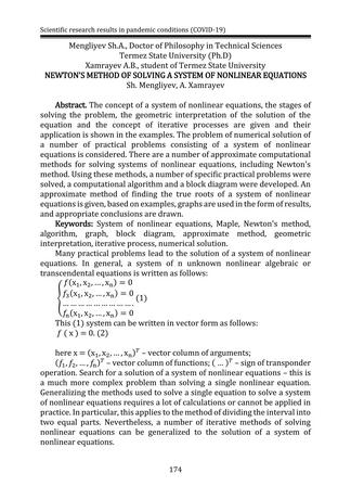
and go to step 2.In calculations
(2) of a system of nonlinear equations
f (x) functions and their derivatives
the matrix W (x) is clearly given,
in which case it is a block diagram of the
solution
of the system As shown in Figure 1.
Figure 1. System of nonlinear equations
algorithm of Newton's method for
solving 𝑓(𝑥) the vector-function x is
continuously differentiable up to twice
around the root and the Jacob matrix 𝑊(𝑥)
the
non-specific,
multidimensional
Newtonian
method
has
a
quadratic
approximation:
|𝑥
(𝑘+1)
− 𝑥| < 𝐶 |𝑥
(𝑘)
− x |
2
We emphasize that the successful
selection of the initial approximation is
important to ensure the approximation of the
method. As the number of equations
increases and their complexity increases, the
area of convergence narrows.
Special case. In computational practice, n = 2 is the most common. Do
this, for example 𝑓(𝑧) = 0 can also be seen in finding the complex roots of a
nonlinear equation. Indeed, if this
𝑓
1
(𝑥, 𝑦) = 𝑅𝑒 ( 𝑓( 𝑥 + 𝑗𝑦 )) and 𝑓
2
(𝑥, 𝑦) = 𝐼𝑚 ( 𝑓( 𝑥 + 𝑗𝑦 ))

Scientific research results in pandemic conditions (COVID-19)
177
If we introduce the functions, z is the real part of the complex root x and
the abstract part y is the approximate solution of the following two unknown
systems of two nonlinear equations:
{
𝑓
1
( 𝑥, 𝑦 ) = 0;
𝑓
2
( 𝑥, 𝑦 ) = 0,
(8)
using Newton's method to calculate this approximation 𝜀 let's do it with
precision.
D belongs to the field 𝑋
0
( 𝑥
0
𝑦
0
) - we choose the zero approximation.
From (5) we can construct the following system of linear algebraic
equations:
𝜕𝑓
1
𝜕𝑥
( 𝑥 − 𝑥
0
) +
𝜕𝑓
1
𝜕𝑦
( 𝑦 − 𝑦
0
) = − 𝑓
1
( 𝑥
0,
𝑦
0
)
𝜕𝑓
2
𝜕𝑥
( 𝑥 − 𝑥
0
) +
𝜕𝑓
2
𝜕𝑦
( 𝑦 − 𝑦
0
) = − 𝑓
2
( 𝑥
0,
𝑦
0
) (9)
We enter the following definitions:
𝑥 − 𝑥
0
= 𝛥𝑥
0
, 𝑦 − 𝑦
0
= 𝛥𝑦
0
(10)
(9) system 𝛥𝑥
0
, 𝛥𝑦
0
for example, using the Kramer method. We write
Kramer's formulas as follows:
𝛥𝑥
0
=
𝛥
1
𝐽
, 𝛥𝑦
0
=
𝛥
2
𝐽
, (11)
where (9) the main determinant of the system is:
𝑱 = |
𝜕 𝑓
1
(𝑥
0
,𝑦
0
)
𝜕 x
𝜕 𝑓
1
(𝑥
0
,𝑦
0
)
𝜕 y
𝜕 𝑓
2
(𝑥
0
,𝑦
0
)
𝜕 x
𝜕 𝑓
2
(𝑥
0
,𝑦
0
)
𝜕 y
| ≠ 0, (12)
(9) The auxiliary determinants of the system are as follows:
𝛥
1
= ||
−𝑓
1
(𝑥
0
, 𝑦
0
)
𝜕 𝑓
1
(𝑥
0
, 𝑦
0
)
𝜕 y
− 𝑓
2
(𝑥
0
, 𝑦
0
)
𝜕 𝑓
2
(𝑥
0
, 𝑦
0
)
𝜕 y
|| ; 𝛥
2
= |
𝜕 𝑓
1
(𝑥
0
, 𝑦
0
)
𝜕 x
−𝑓
1
(𝑥
0
, 𝑦
0
)
𝜕 𝑓
1
(𝑥
0
, 𝑦
0
)
𝜕 x
−𝑓
2
(𝑥
0
, 𝑦
0
)
|.
𝛥𝑥
0
, 𝛥𝑦
0
Substituting the found values of (10) into (9) of the system
𝑋
1
= (𝑥
1
, 𝑦
1
)- find the components of the first approximation:
𝑥
1
= 𝑥
0
+ 𝛥𝑥
0
, 𝑦
1
= 𝑦
0
+ 𝛥𝑦
0
. (13)
We check the fulfillment of the following condition:
𝒎𝒂𝒙 ( |𝛥𝑥
0
|, |𝛥𝑦
0
|) ≤ 𝜀 (14)
if this condition is met, then 𝑋
1
= (𝑥
1
, 𝑦
1
) we stop considering the first
approximation (9) as an approximate solution of the system. If condition
(14) is not met, then 𝑥
0
= 𝑥
1
, 𝑦
0
= 𝑦
1
we construct a new system of linear
algebraic equations (9). Take it off, 𝑋
2
= (𝑥
2
, 𝑦
2
)- we find a tumor near the
second. We check the solution with respect to (14). If this condition is met,
then (9) is an approximate solution of the system 𝑋
2
= (𝑥
2
, 𝑦
2
) we accept.
If condition (14) is not met, then 𝑥
1
= 𝑥
2
, 𝑦
1
= 𝑦
2
that is 𝑋
3
= (𝑥
3
, 𝑦
3
) we

Scientific research results in pandemic conditions (COVID-19)
178
create a new (1.8) system to find, and so on. A block diagram of solving this
system is shown in Figure 2.
Figure 2. Newton's block diagram of the approximate solution of a
system of two nonlinear equations with two unknowns.
1-for example. This
{
𝑓
1
(x, y) = 𝑥
5
+ 𝑦
3
− 𝑥𝑦 − 1 = 0;
𝑓
1
(x, y) = 𝑥
2
y + 𝑦 − 2 = 0.
the zero approximation of the system of equations𝑋
0
( 𝑥
0
, 𝑦
0
) =
( 2 ; 2 ) that is its exact solution X = ( x , y ) = (1; 1) using Newton's method.
Solution: The process of solving an example, the iterations in iterations
𝑋
k
= (𝑥
k
, 𝑦
k
) If you gain 𝛥𝑋
k
= ( 𝛥𝑥
k
, 𝛥𝑦
k
) as in the following table:
k 𝑥
k
𝑦
k
|𝑋
k
− 𝑋|
|𝛥𝑋
k
|/|𝛥𝑋
k−1
|
2

Scientific research results in pandemic conditions (COVID-19)
179
0 2,000000000 2,000000000
1,414213562
-
1 1,693548387 0,890322581
0,702167004
0,351
2 1,394511613 0,750180529
0,466957365
0,947
3 1,192344147 0,82284086
0,261498732
1,199
4 1,077447418 0,918968807
0,112089950
1,639
5 1,022252471 0,976124950 0,032637256
0,032637256
6 1,002942200 0,996839728 4,317853366E -
3
4,054
7 1,000065121 0,999930102 9,553233627E-5 9,553233627E-5
8 1,000000033 0,999999964 0,999999964
5,337
9 1,000000000 1,000000000 1,272646866E-
14
5,363
These results show that the iteration process is very fast - a solution of
up to seven digits after the comma is obtained after eight iterations. A
system of given equations
𝐵 = (
0,032 0,0
0,0 0,9
)
if we solve it by the iteration method with the initial approximation,
then the solution obtained with the comparative error is obtained after 247
iterations.
The numbers in the last column of the table confirm that the method has
a quadratic approximation.
Indeed, | 𝛥𝑋
k
| ≈ 𝐶 | 𝛥𝑋
k−1
|
2
the connection is located close enough
around the root that the constant C is large enough: 𝐶 ≈ 5,4. If the number
of equations in the system of equations increases, then Jacob
we can see that the computational efficiency of Newton's method
decreases due to the difficulty of calculating the matrix. If we look at the one-
dimensional situation, there it is 𝑓(𝑥) and 𝑓
′
(𝑥) The difficulty of calculating
is almost the same. In the N-dimensional case 𝑓
𝑖
′
(𝑥) to calculate 𝑛
2
per
calculation is required, which 𝑓
𝑖
(𝑥) means that it is several times more
difficult to calculate n times.
2-Example. The following
{
F(x, y) = 2𝑥
3
− 𝑦
2
− 1 = 0
G (x, y) = 𝑥 𝑦
3
− 𝑦 − 4 = 0
approximate the solution of the system in Newton's method.
Solution: Initial approximation graphically or selectively 𝑥
0
=
1,2 𝑦
0
= 1,7 be identified. In that case
𝑱 (𝑥
0
, 𝑦
0
) = |
6𝑥
2
− 2𝑦
𝑦
3
3𝑥𝑦
2
− 1
|,
demak
𝑱 (1,2; 1,7) = |
8,64 − 3,40
4,91 9,40
| =
97,910, Abbreviation to formula (13)

Scientific research results in pandemic conditions (COVID-19)
180
{
𝑥
1
= 1,2 −
1
97,91
|
−0,424 − 3,40
0,1956 9,40
| = 1,2 + 0,0349 = 1,2349
𝑦
1
= 1,7 −
1
97,91
|
8,64 − 0,434
4,91 0,1956
| = 1,7 − 0,0390 = 1,6610
Continuing the calculations in the same way,
𝑥
1
= 1,2343 𝑦
1
= 1,6615
In this example, we can see from the following Maple program and
graphs that the system of equations has a single real solution (Figure 3):
> plots[implicitplot]({2*x^3-y^2-1=0,x*y^3-y-4=0},x=-2..2,y=-3..3);
solve({2*x^3-y^2-1=0,x*y^3-y-4=0},{x,y});
allvalues(%);
evalf(%);
{ x = 1.234274484, y = 1.661526467 }
Figure 3. Graphs of functions in a system of equations given in the
example drawn in Maple
Important results of his work are:
1. the solution of a system of nonlinear equations is much more
complicated, and the problem is a perfectly unsolved problem of
computational mathematics; 2. The initial problem of solving a system of
nonlinear equations is the study of the existence, number and interval of
solutions of a system of nonlinear equations, which are explained by solving
specific examples;
3. the problem of finding the separated root of a system of nonlinear
equations has been described in several approximate ways, explained by the
solutions of concrete examples;
4. the approximate methods of finding the roots of a system of nonlinear
equations have been studied from simple to complex and with their special
cases, which has made it possible to shed more light on the subject;
5The existence of real solutions of a system of equations, their number,
the problem of finding the intervals in which these solutions lie, was studied

Scientific research results in pandemic conditions (COVID-19)
181
by drawing a graph of the functions of a system of nonlinear equations using
the Maple package;
6. Newton's method is one of the most effective methods for solving a
system of nonlinear equations, but its scope is very small;
7. The Newtonian method has a quadratic approximation rate;
Thus, the problem of solving a system of nonlinear equations depends
on the type of practical problem, the choice of the correct approximate
method and the initial condition, the effective use of these methods.
References:
1.O’zbekiston Respublikasi Prezidentining 2002 yil 31 maydagi PF-
3080-son
«Kompyuterlashtirishni
rivojlantirish
va
axborot-
kommunikatsiya texnologiyalarini joriy etish to’g’risida»gi Farmoni. –
Toshkent, 2002 yil 31 may.
2.O’zbekiston Respublikasi Vazirlar Mahkamasining 2002.06.06 dagi
200-sonli qarori. – Toshkent, 2002.
3. Абдухамидов А. У., Худойназаров С. Ҳисоблаш усулларидан
амалиёт ва лаборатория машғулотлари. – Тошкент: Ўқитувчи, 1995.
4.Алексеев Е.Р., Чеснокова О.В. Решение задач вычислительной
математики в пакетах Mathcad, Mathlab, Maple (Самоучитель). – М.: НТ
Пресс, 2006. – 496 с.
5.Бахвалов Н.Н. Численные методы. М.: Наука, 1975.
6.Бахвалов Н. С., Жидков Н. П., Кобелков Г. М. Численные методы. –
М.: Лаборатория базовых знаний, 2002. – 600 с.
7.Воробьева Г.К., Данилова А.Н. Практикум по вычислительной
математике. – М: Высшая школа, 1990.
8.Говорухин
В.Н.,
Цибулин
В.Г.
Введение
в
Maple
V.
Математический пакет для всех. - М.: Мир, 1997.
9.Демидович
Б.П.,
Марон
И.А.
Основы
вычислительной
математики. М.: Наука, 1966.
10.Дьяконов В.П. Maple 6: учебный курс. - СПб.: Питер, 2001.
11.Исраилов М.И. Ҳисоблаш усуллари. 1 - қисм. – Тошкент:
Ўқитувчи, 2003.
12.Исраилов М.И. Ҳисоблаш усуллари. 2 - қисм. – Тошкент:
Ўқитувчи, 2004.
13.Калиткин Н.Н. Численные методы. М.: Наука, 1978.
14.Копченова Н.В., Марон И. А. Вычислителная математика в
примерах и задачах. – М.: Наука, 2008. – 368 с.
15.Крылов В.И., Бобков В.В., Монастырский П.И. Вычислительные
методы. М.: Наука, 1976.
16.Манзон Б.М. Maple V Power Edition. - М.: Филинъ, 1998.

Scientific research results in pandemic conditions (COVID-19)
182
17.Сборник задач по методам вычислений. Учебное пособие / Под
ред. П.И.Монастырного. – 2-е изд. – Мн.: Университецкое, 2000. – 311 c.
Mengliyev Sh.A., Doctor of Philosophy in Technical Sciences
Termez State University (Ph.D)
Xamrayev A.B., student of Termez State University
TECHNOLOGY FOR CREATING A DEVICE FOR LAMINAR FLOW OF WATER
IN PIPES
Sh. Mengliyev A. Xamrayev
Abstract: The article discusses the mathematical modeling of the
movement of viscous incompressible fluids through a bundle of tubes
located inside the outer pipe. The laminar and turbulent modes of this
movement are considered, and the physical meaning of their occurrence is
also analyzed. The fluid flow through n tubes of length L and radius r located
inside the outer tube is considered. Calculation formulas are derived for
calculating the maximum velocity of this flow, the volume of fluid passing
through the cross section of the tube, the coefficient of resistance to friction
in the tube along the length of the flow, and also the maximum value of the
tangential stress. The results of the study of the relationship of the
coefficient of resistance to friction in the tube with the Reynolds number are
presented. A description is given of a device created according to the results
of a study that brings the disordered flow of liquids into a laminar state.
Keywords: Reynolds number, laminar flow, turbulent flow, parabolic
flow, friction force, integral, coordinate, pipe, viscosity, density, main flow
velocity, average speed, maximum speed, radius, Hooke, Gegin, Poiseuille,
Darcy-Weisbach, fluid volume, drag coefficient.
The motion of real fluids is often very different from that of laminar flow.
They have a special property called turbulence. As the Reynolds number
increases in real fluid flows in pipes, channels, and boundary layers, the
transformation of a laminar-shaped flow into a turbulent flow is clearly
observed. This transition of laminar flow to turbulent flow is sometimes
called turbulence, which is fundamental in the whole field of
hydrodynamics. Initially, such a transition was observed in the flow of
straight pipes and channels.
Information on the forces acting on a fluid for flow in a cylindrical tube
is given in the article [2; pp. 36-47].
Consider the motion of a tube of constant diameter along its entire
length and the flow of fluid through n tubes of length L and radius r placed